譯者 | 李睿
審校 | 重樓
零日攻擊是當前網絡安全領域最具破壞性的威脅之一,它們利用此前未發現的漏洞入侵,能夠繞過現有的入侵檢測系統(IDS)。傳統的基于簽名的入侵檢測系統(IDS)依賴于已知攻擊模式構建防御規則,因此在此類攻擊面前往往失效。為了檢測這種零日攻擊,人工智能模型需要了解正常的網絡行為模式,并自動識別并標記偏離正常模式的異常行為。
去噪自編碼器(DAE)是一個很有應用前景的解決方案,作為一種無監督深度學習模型,DAE 的核心目標是學習正常網絡流量的穩健特征表示。其核心理念是:在模型訓練過程中,先對輸入的正常網絡流量數據加入輕微噪聲(即“破壞”數據),再迫使模型學習從帶噪數據中重建出原始的“干凈數據”。這迫使其捕捉數據的本質特征,而不是記憶噪聲。一旦遭遇未知的零日攻擊,損失函數(即重建誤差)將會激增,從而實現異常檢測。本文將探討在UNSW-NB15數據集上如何使用DAE進行零日攻擊檢測。
去噪自動編碼器的核心理念
在去噪自編碼器的運作機制中,我們在將輸入數據傳入編碼器之前,會主動向其注入噪聲。隨后,模型的目標是學習從含噪輸入中重構出純凈的原始數據。為了鼓勵模型關注有意義的特征而不是細節,使用隨機噪聲破壞輸入數據。其數學表達式如下:

圖1損失函數
重建損失也稱為損失函數,它評估原始輸入數據x和重構輸出數據x?之間的差異。重建誤差越低,表明模型越能忽略噪聲干擾,并保留輸入數據的核心特征。下圖展示了去噪自編碼器(DAE)的結構示意圖。

圖2 去噪自編碼器的結構示意圖
示例:二元輸入案例
對于二元輸入(x∈{0,1}),以概率q隨機翻轉某一位或將其置零,否則保持不變。如果允許模型以含噪輸入x為目標最小化誤差,模型將只學會簡單復制噪聲。但由于強制其重構真實值x,模型必須從特征間的關聯中推斷缺失信息。這使得去噪自編碼器能夠突破單純記憶的局限,學習輸入數據的深層結構,從而構建出具有噪聲穩健性的模型,并在測試階段展現出更強的泛化能力。在網絡安全領域,去噪自編碼器可以有效檢測偏離正常模式的未知攻擊或零日攻擊。
案例研究:使用去噪自編碼器檢測零日攻擊
這個示例演示了去噪自動編碼器如何檢測UNSW-NB15數據集中的零日攻擊。訓練模型在不受異常數據影響的情況下學習正常流量的底層結構。在推理階段,模型可以評估顯著偏離正常模式的網絡流量(例如零日攻擊相關流量),這些異常流量會產生高重建誤差,從而實現異常檢測。
步驟1.數據集概述
UNSW-NB15數據集是用于評估入侵檢測系統性能的一個基準數據集,包含正常流量樣本及九類攻擊流量(如Fuzzers、Shellcode、Exploits等)。為了模擬零日攻擊,只使用正常流量進行訓練,并單獨保留Shellcode攻擊用于測試,從而確保模型能夠針對未知攻擊行為進行評估。
步驟2.導入庫并加載數據集
導入必要的庫并加載UNSW-NB15數據集。然后執行數字預處理,分離標簽和分類特征,并僅聚焦正常流量進行訓練。
python
import pandas as pd
import numpy as np
import matplotlib.pyplot as plt
from sklearn.model_selection import train_test_split
from sklearn.preprocessing import StandardScaler, OneHotEncoder
from sklearn.compose import ColumnTransformer
from sklearn.metrics import roc_curve, auc
import tensorflow as tf
from tensorflow. keras import layers, Model
from tensorflow. keras.callbacks import EarlyStopping
# Load UNSW-NB15 dataset
df = pd. read_csv("UNSW_NB15.csv")
print ("Dataset shape:", df. shape)
print (df [['label’, ‘attack cat']].head())
輸出:
Dataset shape: (254004, 43)
First five rows of ['label','attack_cat']
     label     attack_cat
 0      0          Normal
 1      0          Normal
 2      0          Normal
 3      0          Normal
 4      1         Shellcode
輸出顯示數據集有254,004行和43列。標簽0表示正常流量,1表示攻擊流量。第五行是Shellcode攻擊,使用它來檢測零日攻擊。
步驟3.預處理數據
python
# Define target
y = df['label']
X = df.drop(columns=['label'])
# Normal traffic for training
normal_data = X[y == 0]
# Zero-day traffic (Shellcode) for testing
zero_day_data = df[df['attack_cat'] == 'Shellcode'].drop(columns=['label','attack_cat'])
# Identify numeric and categorical features
numeric_features = normal_data.select_dtypes(include=['int64','float64']).columns
categorical_features = normal_data.select_dtypes(include=['object']).columns
# Preprocessing pipeline: scale numerics, one-hot encode categoricals
preprocessor = ColumnTransformer([
    ("num", StandardScaler(), numeric_features),
    ("cat", OneHotEncoder(handle_unknown="ignore", sparse=False), categorical_features)
])
# Fit only on normal traffic
X_normal = preprocessor.fit_transform(normal_data)
# Train-validation split
X_train, X_val = train_test_split(X_normal, test_size=0.2, random_state=42)
print("Training data shape:", X_train.shape)
print("Validation data shape:", X_val.shape)
輸出:
Training data shape:    (160000, 71)
Validation data shape:  ( 40000, 71)
在移除數據標簽之后,僅保留良性樣本(即標簽i==0的樣本)。數據集中包含37個數值型特征,以及4個經過獨熱編碼處理的分類型特征——經編碼后,分類型特征轉化為多個二元特征,最終使得輸入數據的總維度達到71維。這些特征共同構成了總計71個維度的輸入。
步驟4.定義優化后的去噪自編碼器(DAE)
在輸入中加入高斯噪聲,以迫使網絡學習具有穩健的特征。批量歸一化可以穩定訓練過程,而小型瓶頸層(16個單元)則有助于形成緊湊的潛在表征。
Python
input_dim = X_train. shape [1]
inp = layers.Input(shape=(input_dim,))
noisy = layers. GaussianNoise(0.1)(inp)  # Corrupt input slightly
# Encoder
x = layers.Dense(64, activation='relu')(noisy)
x = layers. BatchNormalization()(x)  # Stabilize training
bottleneck = layers.Dense(16, activation='relu')(x)
# Decoder
x = layers.Dense(64, activation='relu')(bottleneck)
x = layers. BatchNormalization()(x)
out = layers.Dense(input_dim, activation='linear')(x)  # Use linear for standardized input
autoencoder = Model(inputs=inp, outputs=out)
autoencoder. compile(optimizer='adam', loss='mse')
autoencoder.summary()
輸出:
Model: "model"
_________________________________________________________________
Layer (type)                        Output Shape                          Param #
=================================================================
input_1 (InputLayer)                [(None, 71)]                             0
gaussian_noise (GaussianNoise)      (None, 71)                        0
dense (Dense)                       (None, 64)                                4,608
batch_normalization (BatchNormalization) (None, 64)        128
dense_1 (Dense)                     (None, 16)                              1,040
dense_2 (Dense)                     (None, 64)                               1,088
batch_normalization_1 (BatchNormalization) (None, 64)     128
dense_3 (Dense)                     (None, 71)                               4,615
=================================================================
Total params: 11,607
Trainable params: 11,351
Non-trainable params:   256
步驟5.使用提前停止法訓練模型
Early stopping to avoid overfitting
es = EarlyStopping(monitor='val_loss', patience=3, restore_best_weights=True)
print("Training started...")
history = autoencoder.fit (
    X_train, X_train,
    epochs=50,
    batch_size=512,  # larger batch for faster training    validation_data=(X_val, X_val),
    shuffle=True,
    callbacks=[es]
)
print ("Training completed!")
訓練損失曲線
plt.plot(history.history['loss'], label='Train Loss')
plt.plot(history.history['val_loss'], label='Val Loss')
plt.xlabel("Epochs")
plt.ylabel("MSE Loss")
plt.legend()
plt.title("Training vs Validation Loss")
plt.show()
輸出:
Training started...
Epoch 1/50
313/313 [==============================] - 2s  6ms/step - loss: 0.0254 - val_loss: 0.0181
Epoch 2/50
313/313 [==============================] - 2s  6ms/step - loss: 0.0158 - val_loss: 0.0145
Epoch 3/50
313/313 [==============================] - 2s  6ms/step - loss: 0.0123 - val_loss: 0.0127
Epoch 4/50
313/313 [==============================] - 2s  6ms/step - loss: 0.0106 - val_loss: 0.0108
Epoch 5/50
313/313 [==============================] - 2s  6ms/step - loss: 0.0094 - val_loss: 0.0097
Epoch 6/50
313/313 [==============================] - 2s  6ms/step - loss: 0.0086 - val_loss: 0.0085
Epoch 7/50
313/313 [==============================] - 2s  6ms/step - loss: 0.0082 - val_loss: 0.0083
Epoch 8/50
313/313 [==============================] - 2s  6ms/step - loss: 0.0080 - val_loss: 0.0086
Restoring model weights from the end of the best epoch: 7.
Epoch 00008: early stopping
Training completed!
步驟6.零日檢測
# Transform datasets
X_normal_test = preprocessor.transform(normal_data)
X_zero_day_test = preprocessor.transform(zero_day_data)
# Compute reconstruction errors
recon_normal = np.mean(np.square(X_normal_test - autoencoder.predict(X_normal_test, batch_size=512)), axis=1)
recon_zero = np.mean(np.square(X_zero_day_test - autoencoder.predict(X_zero_day_test, batch_size=512)), axis=1)
# Threshold: 95th percentile of normal errors
threshold = np.percentile(recon_normal, 95)
print("Threshold:", threshold)
print("False Alarm Rate (Normal flagged as anomaly):", np.mean(recon_normal > threshold))
print("Detection Rate (Zero-Day detected):", np.mean(recon_zero > threshold))
輸出:
Threshold: 0.0121
False Alarm Rate (normal→anomaly): 0.0480
Detection Rate (Shellcode zero-day): 0.9150
將檢測閾值設置為良性流量重建誤差的95%。這意味著在模型對正常網絡流量的檢測中,只有4.8%的正常流量因重建誤差超過閾值而被誤標記為異常(即假陽性)。與此同時,在對Shellcode攻擊流量的檢測中,約91.5%的攻擊流量的重建誤差超過了該閾值,從而被模型準確識別為異常(即真陽性)。
步驟7.可視化
重建誤差直方圖
plt. figure(figsize=(8,5))
plt.hist(recon_normal, bins=50, alpha=0.6, label="Normal")
plt.hist(recon_zero, bins=50, alpha=0.6, label="Zero-Day (Shellcode)")
plt.axvline(threshold, color='red', linestyle='--', label='Threshold')
plt.xlabel("Reconstruction Error")
plt.ylabel("Frequency")
plt.legend()
plt.title("Normal vs Zero-Day Error Distribution")
plt.show()
輸出:
圖3良性流量(藍色)和零日流量(橙色)重建誤差的疊加直方圖
ROC曲線
python
y_true = np.concatenate([np.zeros_like(recon_normal), np.ones_like(recon_zero)])
y_scores = np.concatenate([recon_normal, recon_zero])
fpr, tpr, _ = roc_curve(y_true, y_scores)
roc_auc = auc(fpr, tpr)
plt.plot(fpr, tpr, label=f"AUC = {roc_auc:.2f}")
plt.plot([0,1],[0,1],'--')
plt.xlabel("False Positive Rate")
plt.ylabel("True Positive Rate")
plt.legend()
plt.title("ROC Curve for Zero-Day Detection")
plt.show()
輸出:
圖3 ROC曲線展示真陽性率與假陽性率的關系,AUC = 0.93
局限性
以下是這種方法的局限性:
- 去噪自編碼器(DAE)可以檢測異常,但無法對攻擊類型進行分類。
- 選擇合適的閾值取決于數據集的選擇,并且可能需要微調。
- 只有在完全使用正常流量訓練時,效果最好。
關鍵要點
- 去噪自編碼器在檢測未見的零日攻擊方面非常有效。
- 批量歸一化、更大的批次大小以及提前停止法提高了訓練穩定性。
- 可視化(損失曲線、誤差直方圖、ROC)使模型行為可解釋。
- 這種方法能夠以混合方式實現,用于攻擊分類或實時網絡入侵檢測系統。
結論
本文展示了如何使用去噪自編碼器(DAE)在UNSW-NB15數據集中檢測零日攻擊。該模型通過學習正常網絡流量的穩健模式,能夠對未見過的攻擊數據中的異常行為進行標記。去噪自編碼器(DAE)為構建現代入侵檢測系統提供了強大的基礎,并可與先進架構或監督分類器結合,構建全面的入侵檢測系統。
常見問題解答
Q1:在UNSW-NB15數據集上使用去噪自動編碼器(DAE)的目的是什么?
A:在UNSW-NB15 數據集上使用去噪自編碼器,目的是檢測網絡流量中的零日攻擊。去噪自動編碼器(DAE)僅在正常流量上訓練,基于高重建誤差識別異常或攻擊流量。
Q2:如何在去噪自動編碼器中添加噪聲?
A:.在訓練過程中,通過向輸入數據添加高斯噪聲來輸入數據。盡管輸入數據被輕微破壞,但訓練自編碼器重建原始的、干凈的輸入數據,從而使其能夠捕捉更穩健和有意義的數據特征表示。
Q3:自編碼器能否對不同的攻擊類型進行分類?
A:自編碼器屬于無監督學習模型,其功能僅為檢測異常,無法對攻擊類型進行分類。它不會區分具體是哪種攻擊,只會識別出偏離正常網絡行為的流量——這類異常流量可能意味著零日攻擊的發生。
Q4:如何進行零日攻擊檢測?
A:在訓練完成后,評估測試樣本的重建誤差。如果流量的誤差超過了設定的閾值(例如正常誤差的95%),就將其標記為異常。在本文的示例中,將Shellcode 攻擊流量視為零日攻擊流量進行檢測。
Q5:在這個例子中為什么稱其為去噪自編碼器
A:之所以稱為去噪自編碼器,主要原因是模型在訓練階段會向輸入數據添加噪聲。這種方法增強了模型的泛化和識別偏差的能力,這是去噪自編碼器的核心理念。
原文標題:Zero-Day Attack Detection using Denoising Autoencoder on UNSW-NB15,作者:Nitin Wankhade